Full-Grid Stability Sweep and Runtime Model

hard_regime_boundary_sweep.md mapped the boundary around the established hard regime. This page extends the grid further in every dimension and adds an empirical model of how long a parameter combination takes to run, fitted from per-combination timing data.

Method

configs/full_stability_sweep.toml:

Parameter	Range	Count
Df	1.4 to 2.6, step 0.1	13
kf	0.5 to 1.5, step 0.1	11
σ (rp_gstd)	1.0, 1.25, 1.5, 1.75	4
N	128 to 1024, step 128	8
seeds	1, 2, 3, 4, 5 (literal, reused across every combination)	5

13 × 11 × 4 × 8 = 4576 combinations × 5 seeds = 22,880 trials, run via benchmarks/stability_sweep.py’s standard retry-inclusive metric: a single seed maps to whether the CLI’s usual internal 20-attempt retry loop finds a valid aggregate (see pairing_frustration.md for how this differs from the single-shot metric used there).

Raw output: benchmark_results/full_stability_sweep/ (summary JSON/CSV under stability_sweeps/; approximately 15,500 generated aggregate .dat files under aggregates/, kept locally outside version control given the data volume).

Results

Success rate vs Df

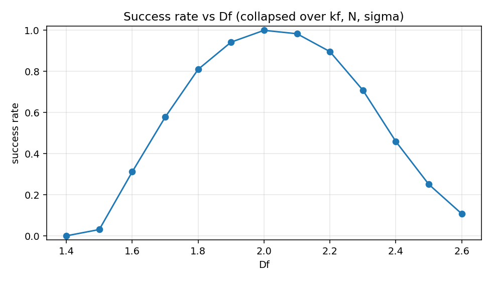
The curve is unimodal, peaking at Df=2.0. This grid’s kf range starts lower (0.5) than earlier characterizations of the safe region, and kf=0.5 already fails at Df=1.8, pulling that Df’s average down to ~81% once included. The apparent “safe” Df region therefore depends on which kf range is averaged over.

Df × kf heatmap

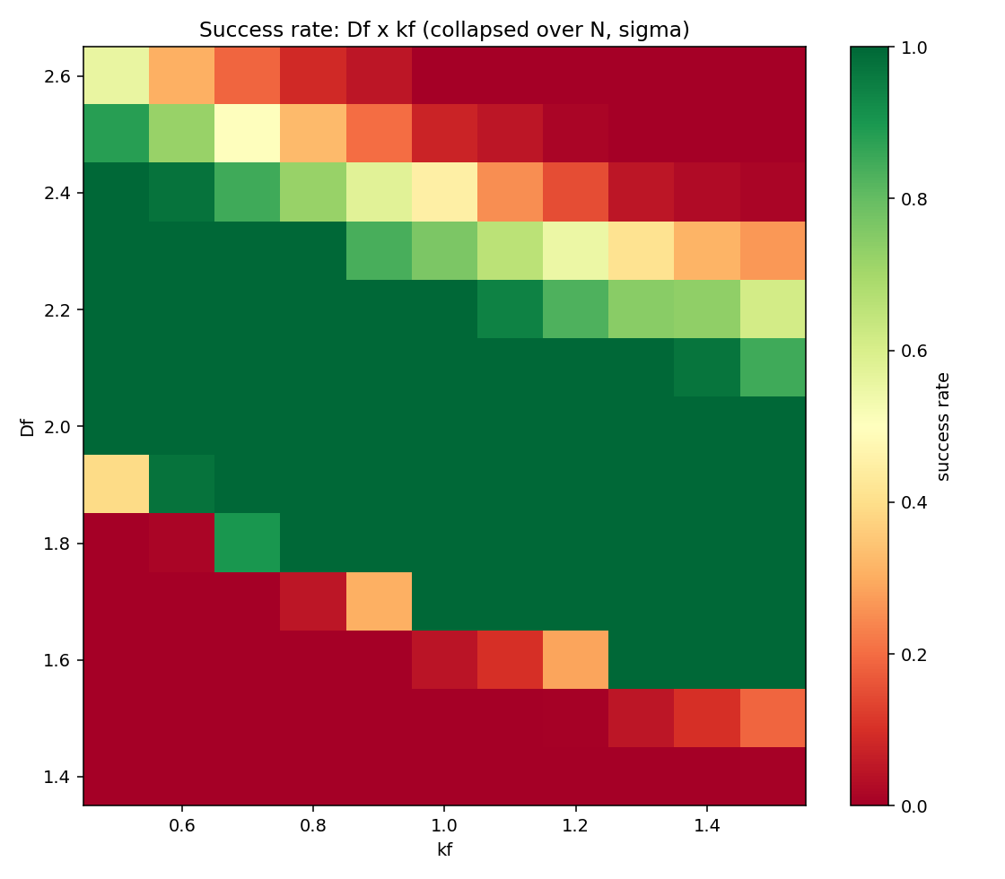
The safe band (Df≈1.8–2.3) is bounded by kf on both sides: higher Df requires lower kf, and vice versa. At the low-Df edge of this grid, Df=1.4 fails at every tested kf from 0.5 to 1.5, suggesting that recovery there requires a substantially larger kf correction than what compensates for high-Df instability in the opposite direction (outside the range tested here).

Success rate vs N and σ

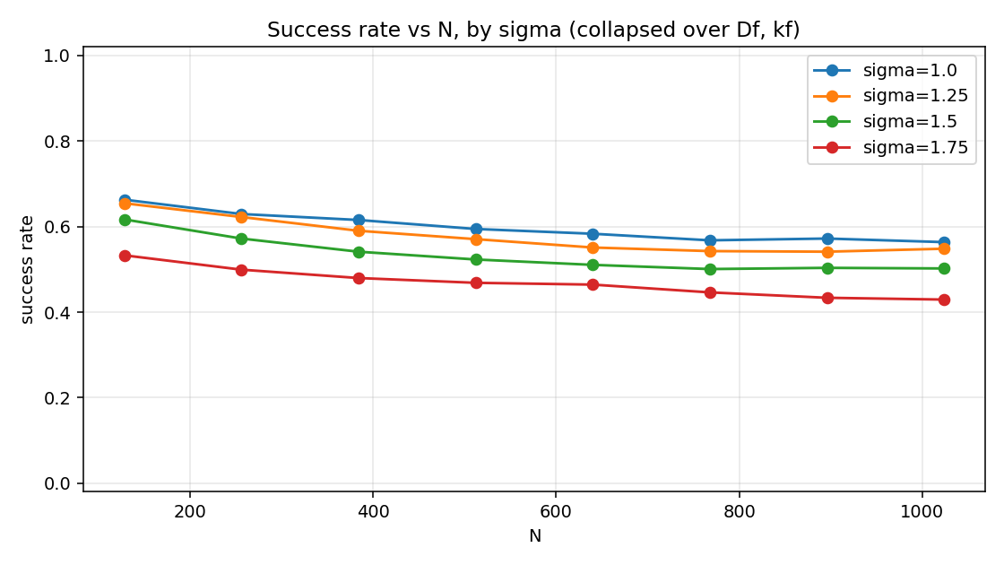
Success rate degrades smoothly and monotonically with both N and σ, with no sharp transitions — consistent with N and σ acting as amplifiers of whatever margin Df/kf leaves rather than as independent failure causes (the same conclusion reached at a finer, boundary-focused grid in hard_regime_boundary_sweep.md).

Empirical runtime model

The summary records only per-combination averages (5 seeds), not individual trial rows (stability_sweep.py’s Dask path does not write raw per-trial output). To keep each fit within a single cost regime, only “clean” combinations are used: all 5 seeds succeeded (2,402 combinations) or all 5 failed (1,985 combinations). The 189 mixed combinations are excluded, since their average blends two different cost profiles — a success stops at the first working attempt, while a failure exhausts all 20 internal retries.

X = (N/kf)^(1/Df), the dimensionless ratio benchmarks/analyze_stability.py uses for stability maps (the number of particle diameters the aggregate must span), is the primary feature alongside raw N. Model: log(runtime_s) = a + b·log(N) + c·log(X), fitted by ordinary least squares.

Regime	n	Equation	R²
Success (5/5 seeds)	2402	runtime_s ≈ exp(-5.58) · N^1.82 · X^-1.37	0.50
Failure, raw (0/5 seeds, incl. timeout-capped)	1985	runtime_s ≈ exp(-1.28) · N^1.17 · X^-0.70	0.69
Failure, uncensored	1397	runtime_s ≈ exp(-1.39) · N^1.12 · X^-0.60	0.48

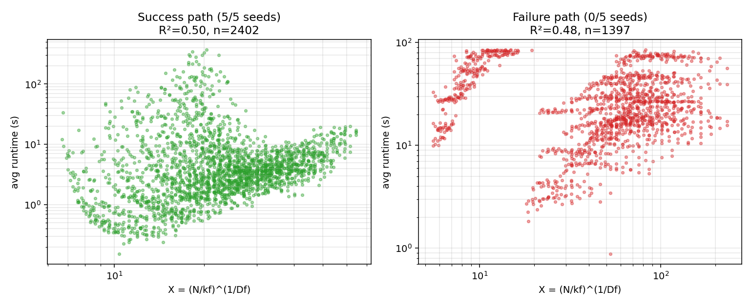
Censoring: trial_timeout=90 in the sweep configuration caps any single trial’s wall-clock budget. 588 of the 1,985 pure-failure combinations (29.6%) hit that cap rather than naturally exhausting all 20 internal retries, visible as a hard ceiling in the raw failure-path scatter. The “raw” fit describes practical wait time under this timeout setting — useful for estimating how long a run takes before giving up — while the “uncensored” fit, restricted to combinations that finished under 85 s on their own, better estimates the algorithmic cost of a failure, at the price of a lower R² (removing the artificially flat ceiling also removes an easy source of apparent fit quality).

Interpreting the exponents: successful runs scale worse than linearly with N (N^1.82), consistent with PCA subclustering and CCA merging both doing more than O(N) work as particle count grows. Failures scale closer to linearly (N^1.1–1.2), since failing trials spend most of their time on the first few CCA rounds before giving up rather than scaling with the full aggregate size. Both regimes show negative exponents on X: within each regime, a combination producing a larger X tends to run faster, not slower. This follows from X not being independent of N (X = (N/kf)^(1/Df)): at fixed N, a large X implies unusually low kf or Df, and such combinations resolve differently rather than more slowly.

The R² of 0.48–0.69 indicates the model explains roughly half to two-thirds of the variance — adequate as an order-of-magnitude estimate for planning a sweep’s compute budget, not as a per-combination predictor. The visibly bimodal structure in both scatter plots (a lower band up to X≈20, a distinct upper band beyond) suggests at least two qualitatively different cost regimes that this three-parameter model does not separate. A Df/kf-aware regression, or a split of the failure population by terminating pipeline stage (PCA vs. CCA), would be the natural refinement if a tighter fit were needed.

Runtime distribution

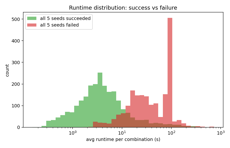
Independent of the model fit: a successful combination in this grid almost always finishes in under 10 s, while a failing one costs anywhere from a few seconds up to the full 90 s timeout, with substantial mass at the cap.

Implementation notes

The sweep took roughly 20 hours wall-clock on a 16-core machine. Two infrastructure issues, visible only at this scale, account for most of that time:

1. get_client()’s local cluster used only 4 of 16 cores. Its docstring states that it “defaults to the number of CPU cores when n_workers is None,” but passing None to LocalCluster does not guarantee that: Dask’s default heuristic also factors in available system memory at cluster start, and selected 4 workers on a 16-core/64 GB machine with a few gigabytes already committed elsewhere (confirmed via the running scheduler’s dashboard). Fixed by resolving n_workers = os.cpu_count() explicitly, appropriate for this purely CPU-bound batch workload.

2. The slowest trials cluster at the tail of a Dask.as_completed() queue: the grid’s largest-N, most extreme Df/kf combinations were both submitted last (sizes is the outermost loop) and individually the most expensive, causing the remaining-time estimate to diverge well past a linear extrapolation from early progress. This is inherent to as_completed() and is better planned around (e.g. submitting the hardest combinations first) than treated as a defect.